Image-specific class saliency

Overview

Saliency map provides a fair summary of pixel importance by studying the positive gradients (of the output class category with respect to an input image) which had more influence to the output.

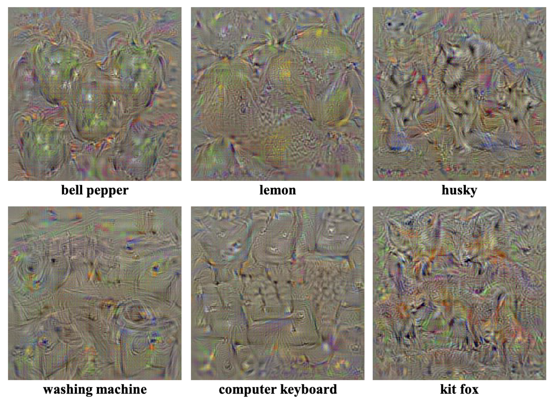xai-saliency-map-visualisation-demo Numerically computed images, illustrating the class appearance models

Motivations

Let $I_{0}$ be a given image, $c$ be a class, and $S_{c} (I)$ be a class score function from the trained CNN (i.e., the CNN classifier function, but without the softmax at its tail). Let $I$ be the image of interest.

The goal is to approximate the class score function for any given image $I$ .

To this end, suppose that $S_{c} (I)$ is linear with respect to $I$ given as:

S_{c} (I) = w^{⊤} I + b_{c}

for some $w$ .

This is, at first glance, obviously very unlikely as CNNs are usually nonlinear.

However, if we assume that $I \approx I_{0}$ , first-order Taylor expansion provides a nice approximation to the original function as:

where S_{c} (I) w = w^{⊤} I + b_{c} = \frac{\partial S _{c}}{\partial I}_{I = I_{0}}

Algorithms

Perform a forwrd pass of $I$ through the CNN.
Compute the gradient of class score of interest with respect to the input pixels:

E_{grad} (I_{0}) = \frac{\partial S _{c}}{\partial I}_{I = I_{0}}

Visualize the gradients.

Limitations

This methods takes the entire neural network as one function and attempts to compute its gradient with respect to the input image.

However, Taylor decomposition is unstable when applied to neutal networks, due to the following reasons.

Shattered gradient: Although $NN (x)$ is typically precise, its gradient often has a lot of random fluctuations and lacks significant information.
Adversarial examples: Minor alterations to the input can lead to substantial modifications in the outputted function value.

References

Simonyan, K., Vedaldi, A., & Zisserman, A. (2013). Deep inside convolutional networks: Visualising image classification models and saliency maps. arXiv preprint arXiv:1312.6034.
https://christophm.github.io/interpretable-ml-book/pixel-attribution.html
Montavon, G., Binder, A., Lapuschkin, S., Samek, W., & Müller, K. R. (2019). Layer-wise relevance propagation: an overview. Explainable AI: interpreting, explaining and visualizing deep learning, 193-209.

🌊