Layer-wise relevance propagation

The notations are slightly different from the original papers; I have added some more index notations to clarify the meanings of each terms.

Overview

Layer-wise Relevance Propagation (LRP) finds relevance scores for individual features in the input data by decomposing the output predictions of the neural network.

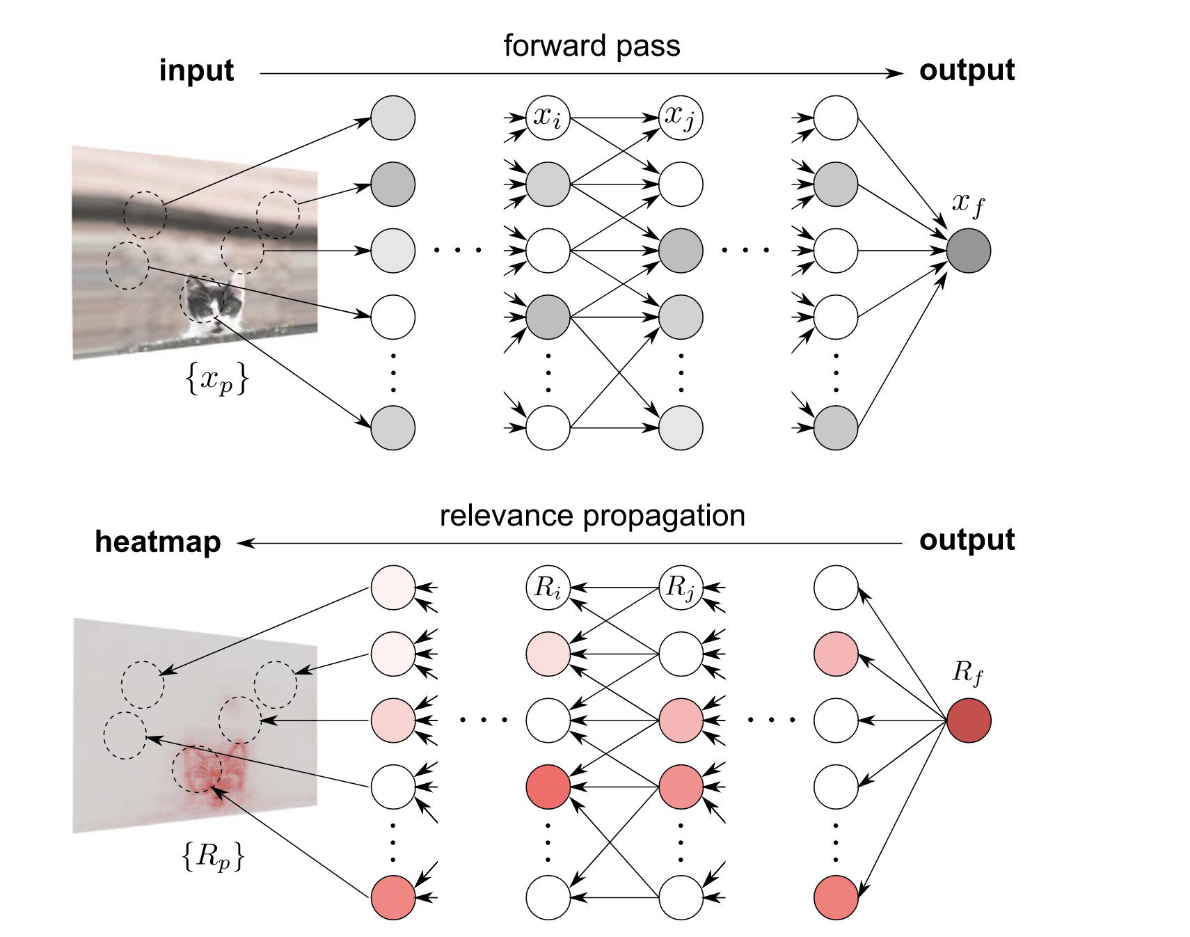
The propagation rule strictly obeys the conservation property: what has been received by a neuron must be redistributed to the lower layer in equal amount. In other words,

$$\sum R_{\text{in}}=\sum R_{\text{out}}$$

for any neuron.

LRP rules

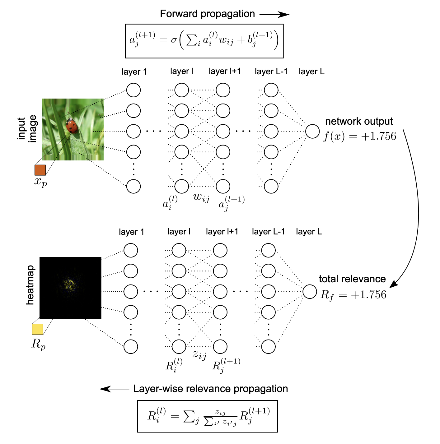
Relevance score propagation at a given layer $l+1$ onto the lower layer $l$ follows:

$$i\in {\mathcal{I}}^{(l)}:R_i^{(l)}=\sum _{j\in {\mathcal{I}}^{(l+1)}}\frac{z_{i,j}}{{\sum }_{k\in {\mathcal{I}}^{(l)}}{z}_{k,j}}{R}_j^{(l+1)}$$

where ${\mathcal{I}}^{(l)}$ is the index set of all neurons in the $l$-th layer.

Consequently,

$$f(x)=\cdots =\sum _{i\in {\mathcal{I}}^{(l)}}{R}_i^{(l)}=\cdots =\sum _{i\in {\mathcal{I}}^{(1)}}{R}_i^{(1)}$$

where $f(x)$ is the prediction of the neural network for an input $x$.

The quantity $z_{i,j}$ indicates how much neuron $i$ has contributed to make neuron $j$ relevant. There are several possible variants of LRP according to the choice of $z_{i,j}$.

Basic rule (LRP-0)

LRP-0 redistributes relevance score proportionally to the contributions of each input to the neuron activation.

Let $a_i$ be the activation of neuron $i$, and $w_{i,j}$ be the weight parameter applied to neuron $i$ to neuron $j$ of subsequent layer. Then, LRP-0 is defined as

$$z_{i,j}=a_i{w}_{i,j}$$

or in other words,

$$i\in {\mathcal{I}}^{(l)}:R_i^{(l)}=\sum _{j\in {\mathcal{I}}^{(l+1)}}\frac{a_i{w}_{i,j}}{{\sum }_{k\in {\mathcal{I}}^{(l)}}{a}_k{w}_{k,j}}{R}_j^{(l+1)}$$

Note that the sum runs over all neurons of the lower layer, including that of the bias term.

Although this rule looks intuitive, a uniform application of LRP-0 to the entire network is empirically shown to be equivalent to gradient $\times$ input, where the gradients are usually noisy.

Epsilon rule (LRP-$\epsilon$)

LRP-$\epsilon$ adds a small positive term $\epsilon$ in the denominator.

$$i\in {\mathcal{I}}^{(l)}:R_i^{(l)}=\sum _{j\in {\mathcal{I}}^{(l+1)}}\frac{a_i{w}_{i,j}}{\epsilon +{\sum }_{k\in {\mathcal{I}}^{(l)}}{a}_k{w}_{k,j}}{R}_j^{(l+1)}$$

The term $\epsilon$ absorbs some relevance when the contributions to the activation of neuron $k$ are weak or contradictory (i.e., diminishing the relevance score).

As the term $\epsilon$ becomes bigger, only the most salient explanation factors survive the absorption, resulting in a less noisy explanation.

Gamma rule (LRP-$\gamma$)

LRP-$\gamma$ favours the effect of positive contributions over negative contributions.

$$\begin{array}{rl}i\in {\mathcal{I}}^{(l)}:R\_i^{(l)}& =\sum \_j\in {\mathcal{I}}^{(l+1)}\frac{a\_i(w\_i,j+\gamma w\_{i,j}^{+})}{\sum \_k\in {\mathcal{I}}^{(l)}a\_k(w\_k,j+\gamma w\_{k,j}^{+})}R\_j^{(l+1)}\\ & \\ & =\sum \_j\in {\mathcal{I}}^{(l+1)}\frac{a\_i(w\_{i,j}^{-}+(1+\gamma )w\_{i,j}^{+})}{\sum \_k\in {\mathcal{I}}^{(l)}a\_k(w\_{k,j}^{-}+(1+\gamma )w\_{k,j}^{+})}R\_j^{(l+1)}\end{array}$$

Here, $w_{i,j}^{-}$ and $w_{i,j}^{+}$ denotes the negative and positive parts of $w_{i,j}$, respectively.

The term $\gamma$ quantifies how much the positive contributions are favoured.

The prevalence of positive contributions has a limiting effect on how large positive and negative relevance can grow in the propagation phase, resulting in a more stable explanation.

Deep Taylor decomposition

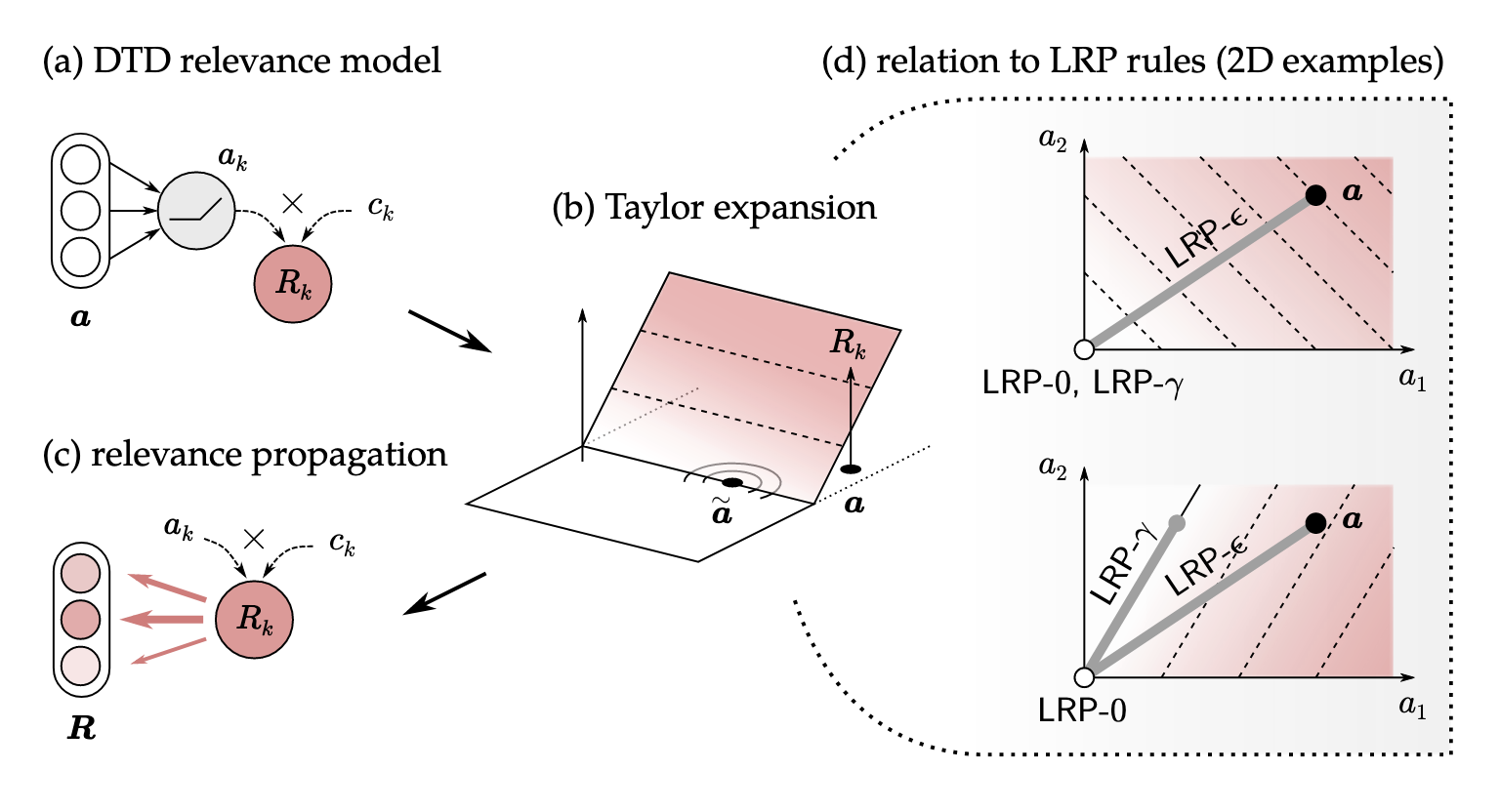
The previous rules can be interpreted with Deep Taylor Decomposition (DTD), which views LRP as a succession of Taylor expansions performed locally at each neuron.

Let ${\mathbf{a}}^{(l)}=(a_1^{(l)},\cdots ,a_{|{\mathcal{I}}^{(l)}|}^{(l)})$ denote the vector of lower-level (layer $l$) activations, and let ${\tilde{\mathbf{a}}}^{(l)}$ be some reference point near ${\mathbf{a}}^{(l)}$. Then,

$$\begin{array}{rl}R\_j^{(l+1)}({\mathbf{a}}^{(l)})& =R\_j^{(l+1)}({\tilde{\mathbf{a}}}^{(l)})+\sum \_i\in {\mathcal{I}}^{(l)}\frac{\partial R\_j^{(l+1)}}{\partial a\_i^{(l)}}|\_{\mathbf{a}}^{(l)}={\tilde{\mathbf{a}}}^{(l)}(a\_i^{(l)}-\tilde{a}\_i^{(l)})+\epsilon \\ & \\ & =R\_j^{(l+1)}({\tilde{\mathbf{a}}}^{(l)})+\sum \_i\in {\mathcal{I}}^{(l)}\left(\left[\nabla R\_j^{(l+1)}({\tilde{\mathbf{a}}}^{(l)})\right]\_i(a\_i^{(l)}-\tilde{a}\_i^{(l)})\right)+\epsilon \end{array}$$

where $\epsilon$ denotes the error term, which consists of the second and higher order terms of the Taylor expansion that are difficult to compute.

Relevance model

By substituting the relevance function $R_j^{(l+1)}$, a closed-form expression can be derived. One popular choice is the modulated ReLU activation:

$$\hat{R}\_j^{(l+1)}({\mathbf{a}}^{(l)})=c\_j\cdot \max \left(0,\sum \_i\in {\mathcal{I}}^{(l)}a\_i^{(l)}w\_i,j\right)$$

where $c_j$ is the modulation term set to satisfy $R_j^{(l+1)}({\mathbf{a}}^{(l)})={\hat{R}}_j^{(l+1)}({\mathbf{a}}^{(l)})$.

Then, the Taylor expansion of ${\hat{R}}_j^{(l+1)}$ can be given as

$$\begin{array}{rl}\hat{R}\_j^{(l+1)}({\mathbf{a}}^{(l)})& =\hat{R}\_j^{(l+1)}({\tilde{\mathbf{a}}}^{(l)})+\sum \_i\in {\mathcal{I}}^{(l)}\left(\left[\nabla \hat{R}\_j^{(l+1)}({\tilde{\mathbf{a}}}^{(l)})\right]\_i(a_i^{(l)}-\tilde{a}\_i^{(l)})\right)+\epsilon \\ & =\hat{R}\_j^{(l+1)}({\tilde{\mathbf{a}}}^{(l)})+\sum \_i\in {\mathcal{I}}^{(l)}\left(c\_j\cdot w\_i,j(a\_i^{(l)}-\tilde{a}\_i^{(l)})\right)\end{array}$$

Here, due to the linearity of $\hat{R}$, $\epsilon =0$ (Recall that $\epsilon$ consists of the second and higher order terms of the Taylor expansion).

Once the reference point $\tilde{\mathbf{a}}$ is chosen, relevance scores can be easily computed because they only consist of first-order terms.

References

• Bach, S., Binder, A., Montavon, G., Klauschen, F., Müller, K. R., & Samek, W. (2015). On pixel-wise explanations for non-linear classifier decisions by layer-wise relevance propagation. PloS one, 10(7), e0130140.
• Montavon, G., Binder, A., Lapuschkin, S., Samek, W., & Müller, K. R. (2019). Layer-wise relevance propagation: an overview. Explainable AI: interpreting, explaining and visualizing deep learning, 193-209.
• Kim, S. W., Kang, S. H., Kim, S. J., & Lee, S. (2021). Estimating the phase volume fraction of multi-phase steel via unsupervised deep learning. Scientific Reports, 11(1), 5902.
• Montavon, G., Lapuschkin, S., Binder, A., Samek, W., & Müller, K. R. (2017). Explaining nonlinear classification decisions with deep taylor decomposition. Pattern recognition, 65, 211-222.