Decoding the Black Box - Insights into Machine Learning Models with Surrogate Analysis

Introduction to Machine Learning Interpretability

In today’s fast-paced AI world, making machine learning models easy to understand, or interpretable, is crucial. Interpretability means explaining a model’s workings in simple terms, turning complex, ‘black box’ models into transparent ones. This is important for many reasons, like ensuring a model works correctly and is used ethically. With the rise of complex deep learning models, interpretability has become both harder and more essential. These advanced models are increasingly used in important decisions, so understanding how they work is not just a technical issue, but a societal one.

According to Das et al., Explainable Artificial Intelligence (XAI) involves tools, techniques, and algorithms that make AI decisions clear and understandable. XAI is key in making AI systems transparent and responsible, ensuring they meet ethical standards and human values. It is not just about technology; it is about making sure AI advancements are clear, responsible, and inclusive.

This project focuses on a particular aspect of XAI: local surrogate models. These models provide insights into the decision making process of algorithms by approximating their behaviour near a specific data point. This method gives us a closer look at why a model makes certain predictions, one case at a time.

Overview of XAI Methods

In this project, we will explore two of the most prominent techniques in the realm of local surrogate models: Local Interpretable Model-agnostic Explanations (LIME) and SHapley Additive exPlanations (SHAP). These methods have gained widespread recognition for their ability to effectively illuminate the inner workings of complex models, thereby enhancing transparency and trust in AI. We will examine these techniques in detail, understand their methodologies, and demonstrate the applications through practical examples.

LIME (Local Interpretable Model-agnostic Explanations)

Surrogate Analysis

Before we dive into LIME, let us talk about the concept of surrogate analysis. In XAI, surrogate analysis refers to the technique of interpreting an existing model using an interpretable surrogate model when the original model to be explained is too complex to interpret.

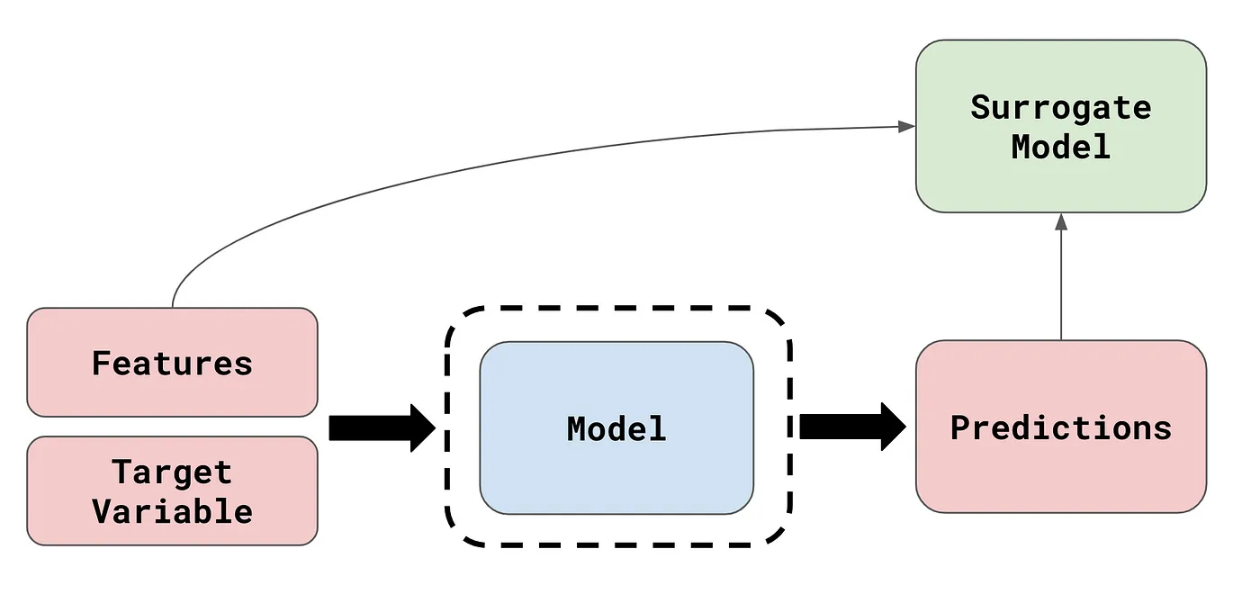
Image Source: What are Model Agnostic Methods?

Surrogate analysis methods are very useful in that they are model-agnostic. However, because they interpret using a surrogate model that is less complex than the original model of interest, they cannot generalise well to the entire dataset, and can only generate accurate explanations for a few specific instances at a time; they only provide a local explanation.

Visualising the Algorithm

The LIME algorithm interprets machine learning models by approximating the model locally around the prediction instance of interest.

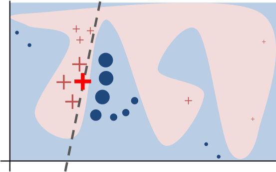
Image Source: “Why Should I Trust You?” Explaining the Predictions of Any Classifier

The algorithm’s intuition is presented in the diagram above. The blue/pink background represents the complex decision function $f$ of the black-box model, which is unknown to LIME and difficult for a linear model to accurately simulate. The instance that is being explained is the bold red cross. LIME gathers samples of instances, uses $f$ to generate predictions, and then measures each prediction’s proximity to the instance being explained (here represented by size). The learned explanation that is faithful locally (but not globally) is indicated by the dashed line.

Now, let us observe the algorithm in action by a step-by-step visualisation.

Preparation of the Dataset and the Model to Explain

First, as a mock example, we generate a 2-dimensional synthetic dataset and train a logistic regression with polynomial features on it.

RAND_SEED = 999
 
X, y = make_classification(
    n_samples=1000, n_features=2, n_informative=2, n_redundant=0, random_state=RAND_SEED
)
X_train, X_test, y_train, y_test = train_test_split(
    X, y, test_size=0.3, random_state=RAND_SEED
)
 
plt.figure(figsize=(10, 6))
plt.scatter(
    X[:, 0], X[:, 1], marker="o", c=y, s=25, edgecolor="k", cmap=plt.cm.coolwarm
)
plt.title("Synthetic Dataset")
plt.xlabel("$x_1$")
plt.ylabel("$x_2$")
plt.show()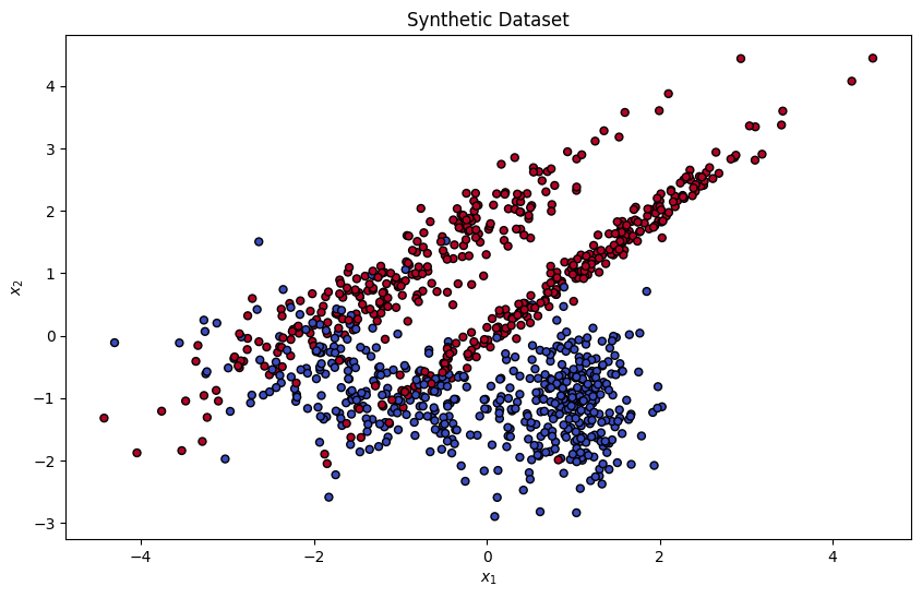

# logistic regression model with polynomial features
polynomial_degree = 5
target_model = Pipeline([
    ("polynomial_features", PolynomialFeatures(degree=polynomial_degree)),
    ("logistic_regression", LogisticRegression(random_state=RAND_SEED))
])
target_model.fit(X_train, y_train)
 
x_min, x_max = X[:, 0].min() - 1, X[:, 0].max() + 1
y_min, y_max = X[:, 1].min() - 1, X[:, 1].max() + 1
xx, yy = np.meshgrid(np.linspace(x_min, x_max, 100), np.linspace(y_min, y_max, 100))
Z = target_model.predict(np.c_[xx.ravel(), yy.ravel()])
Z = Z.reshape(xx.shape)
 
plt.figure(figsize=(10, 6))
plt.contourf(xx, yy, Z, alpha=0.4, cmap=plt.cm.coolwarm)
plt.scatter(X_train[:, 0], X_train[:, 1], c=y_train, s=25, edgecolor='k', cmap=plt.cm.coolwarm)
plt.title("Decision Boundary")
plt.xlabel("$x_1$")
plt.ylabel("$x_2$")
plt.show()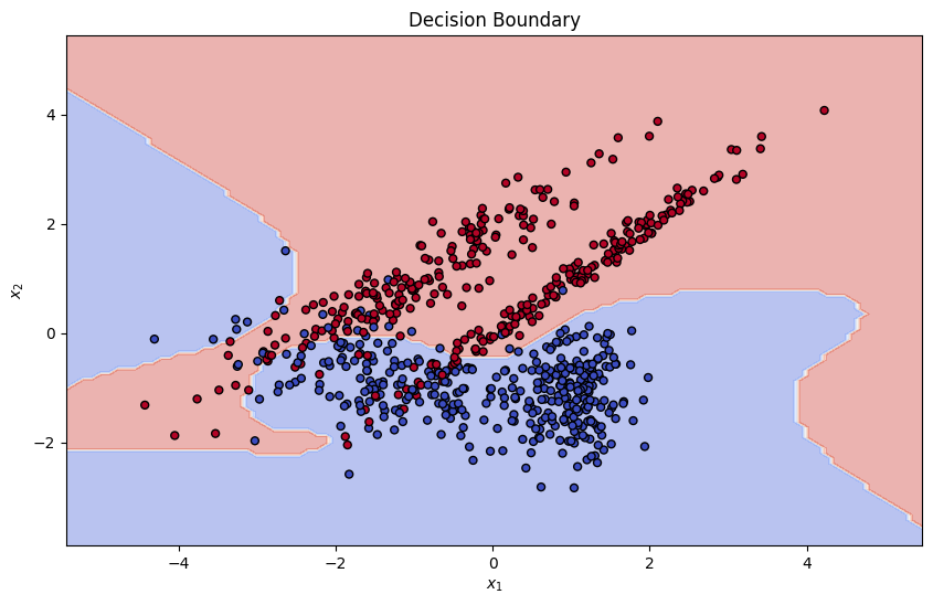

Selection and Perturbation of Data

LIME starts by selecting the instance that needs to be explained, typically a single prediction from the model. It then generates a new dataset consisting of perturbed samples around the selected instance. This is done by adding noise to the features of the instance to create similar, but slightly varied, instances.

probs = target_model.predict_proba(X_test)[:, 1]
 
closest_to_boundary_index = np.argmin(np.abs(probs - 0.5))
instance_to_explain = X_test[closest_to_boundary_index]
 
num_samples = 500
 
# generate perturbed samples by adding random noise drawn from a normal distribution
noise_scale = 0.1 * (X_train.max(axis=0) - X_train.min(axis=0))
perturbed_samples = np.tile(instance_to_explain, (num_samples, 1))
perturbed_samples += np.random.normal(0, noise_scale, size=perturbed_samples.shape)
 
plt.figure(figsize=(10, 6))
plt.scatter(X_train[:, 0], X_train[:, 1], c=y_train, s=10, edgecolor='k', cmap=plt.cm.coolwarm, alpha=0.2)
plt.scatter(perturbed_samples[:, 0], perturbed_samples[:, 1], c='orange', s=25, alpha=1, label='Perturbed Samples')
plt.scatter(instance_to_explain[0], instance_to_explain[1], c='red', s=100, edgecolor='k', label='Instance to Explain')
plt.title("Perturbed Samples")
plt.xlabel("$x_1$")
plt.ylabel("$x_2$")
plt.legend()
plt.show()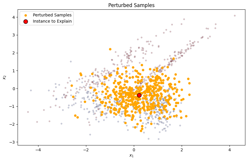

Proximity Function

For each perturbed sample, a proximity measure is calculated to determine its closeness to the original instance. This measure influences the weight of each perturbed sample in the surrogate model. The original paper uses an exponential kernel defined on some distance metric $D$ (e.g. cosine distance, L2 distance) with width $\sigma$:

$${\pi }_x(z)=\exp (-D(x,z{)}^2/{\sigma }^2)$$

as the proximity function.

Here, we shall use the Euclidean distance for the distance metric:

$$D(x,z)=\Vert x-z{\Vert }_2$$

def euclidean_distance(a, b):
    return np.sqrt(np.sum((a - b) ** 2, axis=1))
 
distances = euclidean_distance(perturbed_samples, instance_to_explain.reshape(1, -1))
sigma = distances.std()
proximity_weights = np.exp(-(distances ** 2) / (sigma ** 2))
 
log_proximity_weights = np.log(proximity_weights + 1e-5)
log_proximity_weights_normalized = (log_proximity_weights - log_proximity_weights.min()) / (log_proximity_weights.max() - log_proximity_weights.min())
 
plt.figure(figsize=(10, 6))
plt.scatter(X_train[:, 0], X_train[:, 1], alpha=0)
plt.scatter(perturbed_samples[:, 0], perturbed_samples[:, 1], c=log_proximity_weights_normalized, alpha=0.5, label='Perturbed Samples')
plt.scatter(instance_to_explain[0], instance_to_explain[1], c='red', s=100, label='Instance to Explain', edgecolors='k')
plt.title("Perturbed Samples Proximity")
plt.xlabel("$x_1$")
plt.ylabel("$x_2$")
plt.colorbar(label='Proximity Weights (Normalised, log scale)')
plt.legend()
plt.show()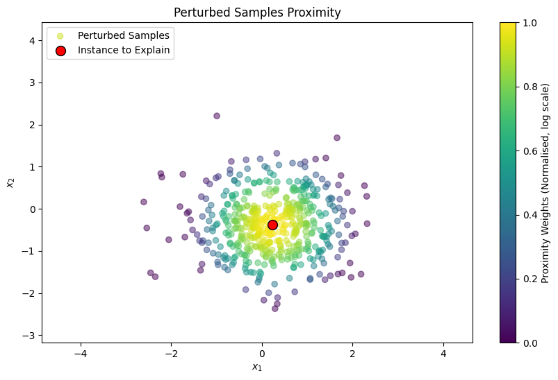

Training the Surrogate Model

A simple, interpretable model (such as linear regression) is trained on this weighted, perturbed dataset. The surrogate model is designed to approximate the predictions of the complex model locally.

Mathematically, local surrogate models with interpretability constraint can be expressed as follows:

$$\xi (x)={\arg \min }_g\mathcal{L}(f,g,{\pi }_x)+\Omega (g)$$

The explanation model for instance $x$ is the surrogate model $g$ that minimises loss $\mathcal{L}$, which measures how close the explanation is to the prediction of the original model $f$, while the model complexity regularising term $\Omega (g)$ is kept low (this ensures that the surrogate model $g$ has low enough complexity to be inherently interpretable). $G$ is the family of possible explanations.

The original paper limits $g$ to a class of linear models, such that $g(z)=w_{g}z$. The loss function is given as a locally weighted square loss:

$$\mathcal{L}(f,g,{\pi }_x)=\sum _{z,z^{\prime }\in \mathcal{Z}}{\pi }_x(z){\left(f(z)-g(z^{\prime })\right)}^2$$

Here, we shall use a ridge regression model as a surrogate model.

target_predictions = target_model.predict(perturbed_samples)
 
surrogate_model = Ridge(alpha=1, fit_intercept=True, random_state=RAND_SEED)
surrogate_model.fit(perturbed_samples, target_predictions, sample_weight=proximity_weights)
 
Z_target = target_model.predict(np.c_[xx.ravel(), yy.ravel()])
Z_target = Z_target.reshape(xx.shape)
 
Z_surrogate = surrogate_model.predict(np.c_[xx.ravel(), yy.ravel()])
Z_surrogate = Z_surrogate.reshape(xx.shape)
 
plt.figure(figsize=(10, 6))
plt.contourf(xx, yy, Z_target, alpha=0.4, cmap=plt.cm.coolwarm,)
plt.contour(xx, yy, Z_surrogate, levels=[0.5], colors='green', linestyles='dashed', label='Surrogate Model')
plt.scatter(X[:, 0], X[:, 1], c=y, s=25, edgecolor='k', cmap=plt.cm.coolwarm)
plt.scatter(instance_to_explain[0], instance_to_explain[1], c='red', s=100, edgecolor='k', label='Instance to Explain')
plt.title("Target and Surrogate Model Decision Boundaries")
plt.xlabel("$x_1$")
plt.ylabel("$x_2$")
plt.legend()
plt.show()

This demonstrates how the ridge regression model, serving as our surrogate, effectively captures and explains the decision-making process of the original model within a local context.

Shapley Additive Explanations

SHAP (SHapley Additive exPlanations) represents a novel approach in the realm of interpretable machine learning, drawing inspiration from game theory to explain the output of machine learning models. While LIME generates explanations by locally approximating the model with simpler, interpretable models, SHAP takes a slightly different approach. It explains predictions by calculating the contribution of each feature to the prediction, using concepts derived from cooperative game theory.

Image Source: SHAP: A game theoretic approach to explain the output of any machine learning model

At the core of SHAP is the Shapley value, a concept from game theory that offers a method to fairly distribute the ‘payout’ (or prediction) among the ‘players’ (or features). SHAP treats each feature as a player in a coalition (the model), where the contribution of each feature to the model’s prediction is similar to a player’s contribution to a game’s total payoff. This way, SHAP looks at every possible group of features to figure out how important each one is, giving a complete and fair view of each feature’s impact.

Shapley Values

Suppose that there is a set $N$ (of $n$ players) and a function $v$ that maps subsets of players to the real numbers: $v:2^N\to \mathbb{R}$, with $v(\varnothing )=0$. The function $v$ means that if $S(\subseteq N)$ is a coalition of players, then the total expected sum of payoffs that the members of $S$ can earn by cooperating is described by $v(S)$, often known as the coalition’s worth.

Now, assuming that all players collaborate, let’s say that we want to distribute the total gains to the players, i.e., find a distribution ${\varphi }_i(v)$ for each player $i$. A definition of a ‘fair’ distribution can be justified through some desriable proeprties.

• Efficiency: The sum of the distribution to each players should equal the value of the grand coalition:

  $$\sum _{i\in N}{\varphi }_i(v)=v(N).$$

• Symmetry: If $i$ and $j$ are two players that satisfies

  $$v(S\cup \{i\})=v(S\cup \{j\})$$

  for every subset $S\subset N$ such that $i\notin S$ and $j\notin S$, then

  $${\varphi }_i(v)={\varphi }_j(v).$$

• Linearity: The distributed gains should match the gains from $v$ and the gains from $w$ if two coalition games defined by gain functions $v$ and $w$ are combined: for every $i\in N$,

  $${\varphi }_i(v+w)={\varphi }_i(v)+{\varphi }_i(w)$$

  and

  $${\varphi }_i(av)=a{\varphi }_i(v)$$

  for any real number $a$.

• Null Player: A player $i$ is null in $v$ if $v(S\cup \{i\})=v(S)$ for all coalitions $S$ that do not contain $i$. If $i$ is a null player, then

  $${\varphi }_i(v)=0.$$

It has been mathematically proven that there exists a unique distribution that satisfies all four properties: the Shapley value! According to the Shapley value, the amount that player $i$ is given in a coalitional game $(v,N)$ is given as follows:

$$\begin{array}{rl}{\varphi }_i(v)& =\sum _{S\subseteq N\setminus \{i\}}\frac{|S|!(n-|S|-1)!}{n!}(v(S\cup \{i\})-v(S))\\ & =\frac{1}{n}\sum _{S\subseteq N\setminus \{i\}}{\left(\genfrac{}{}{0ex}{}{n-1}{n-|S|-1}\right)}^{-1}(v(S\cup \{i\})-v(S))\end{array}$$

SHAP (SHapley Additive exPlanation) Values

We can further extend this concept of Shapley value in terms of interpreting machine learning models. As in LIME, we want to build a surrogate model, an interpretable (local) approximation of the original model. First, let us clarify some notations:

• $f$ is the model we want to explain.
• $M$ is the number of features.
• $\mathcal{X}={\mathbb{R}}^M$ is the original feature space (= input space of $f$). Its elements can be fed to $f$ directly.
• $x^{\ast }\in \mathcal{X}$ is the instance we want to explain.
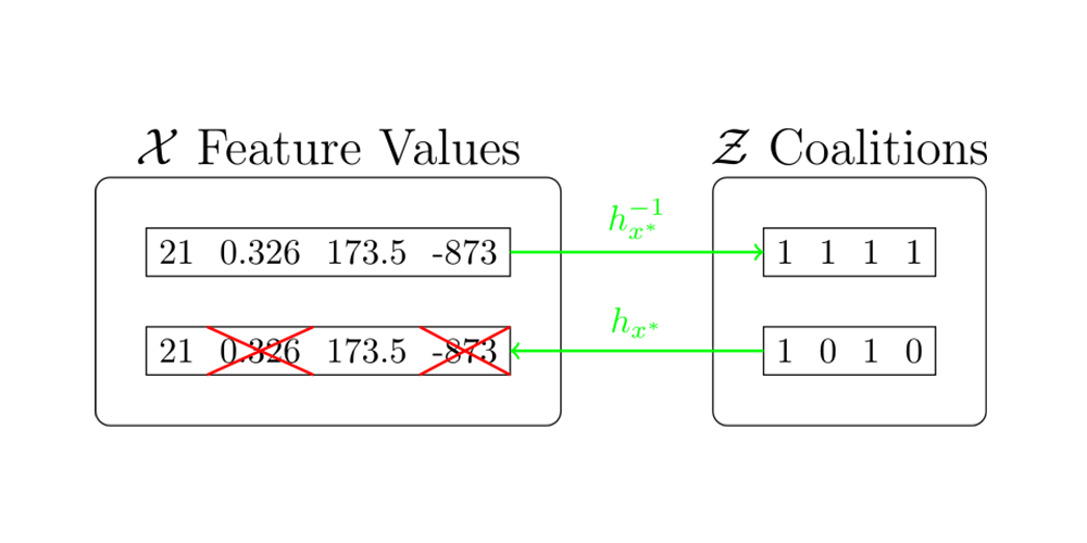
• $\mathcal{Z}=\{0,1{\}}^M$ is the coalition space.
• $z=(z_1,\cdots ,z_M)\in \mathcal{Z}$ is a coalition vector that contains information about which feature is present and which is absent. (The $i$-th feature is present if $z_i=1$, and vice versa.)
• $z_S\in \mathcal{Z}$ is a coalition vector where the set $S$ indicates the nonzero indices. i.e., $$(z_S{)}_i=\{\begin{array}{l}1\text{ if }i\in S\\ 0\text{ otherwise}\end{array}$$
• $z^{\ast }=(1,\cdots ,1)$
• $h_{x^{\ast }}:\mathcal{Z}\to \mathcal{X}$ is a mapping function that maps a coalition to its corresponding input. It satisfies that

$$h_{x^{\ast }}(z^{\ast })=x^{\ast }.$$

For detailed information about the relation between the original feature space and the coalition space, refer to the following diagram.

SHAP proposes the surrogate model $g$ as follows:

$$g(z)={\varphi }_0+\sum _{i=1}^M{\varphi }_i{z}_i$$

where

$${\varphi }_i=\sum _{S\in F_i}\frac{|S|!(M-|S|-1)!}{M!}(f(h_{x^{\ast }}(z_{S\cup \{i\}}))-f(h_{x^{\ast }}(z_S)))$$

Here, $F_i$ is the set of all possible feature combinations that does not contain the feature $i$. ($|F_i|=2^{M-1}$). However, two problems arise when defining SHAP values as above.

• Most machine learning models cannot handle arbitrary patterns of missing input values. They require a full feature set to make predictions, complicating the direct application of Shapley values which inherently involve evaluating the model on various feature subsets.

• To accurately determine each feature’s Shapley value, every possible combination of features must be considered. However, in modern machine learning models where the number of features ($M$) is often very large, computing precise Shapley values for each feature becomes infeasible.

Various methods have been developed to calculate Shapley values, which help explain model predictions using feature subsets. Amongst such methods, KernelSHAP is notable for its versatility, making it a useful tool for understanding machine learning predictions. This project will focus on KernelSHAP due to its wide applicability and thorough interpretative capabilities.

KernelSHAP

KernelSHAP process involves generating feature coalitions, predicting outcomes with the complete model while handling absent features through marginalisation, and then fitting a surrogate model to these predictions.

Let us start by extending the previous notations:

• $\mathcal{D}\subset \mathcal{X}$ is the training dataset.
• For $x=(x_1,\cdots ,x_M)\in \mathcal{D}$ and a set $S$ of indices, a partial representation $x_S$ is defined as: $$x_S=(x_i{)}_{i\in S}$$
• $\overline{S}$ is the complementary set of $S$.

To overcome the first problem, the original paper approximates $f(h_{x^{\ast }}(z_S))$ as follows:

$$\begin{array}{rl}f(h_{x^{\ast }}(z_S))& \approx \mathbb{E}[f(x)|x_S=x_S^{\ast }]\\ & \approx {\mathbb{E}}_{x_{\overline{S}}}[f(x;x_S=x_S^{\ast })]\end{array}$$

Here, features that are not in $S$ (i.e., $x_{\overline{S}}$) are replaced with values randomly sampled from $\mathcal{D}$.

One downside of this approximation is that it assumes the independence between features in the last step. This is the same as assuming that regardless of the composition of the original coalition, the effects of adding a variable to it are always the same. This assumption provides an approach for computing the model prediction with missing values, which resolves the problem of handling absent features.

For example, consider a case with 3 dimensional data, and suppose that we are given $S=\{1,2\}$ (i.e., $\overline{S}=\{3\}$). Then, applying the previous approximation logic,

$$\begin{array}{rl}f(h_{x^{\ast }}(z_{\{1,2\}}))& \approx \mathbb{E}[f(x)|x_1=x_1^{\ast },x_2=x_2^{\ast }]\\ & \approx {\mathbb{E}}_{x_3}[f((x_1^{\ast },x_2^{\ast },x_3))].\end{array}$$

Now, let us observe the algorithm in action with visualisation.

1-dimensional Case

Let us start by generating a synthetic dataset, and a mock model to explain.

np.random.seed(RAND_SEED)
x_dataset = np.random.uniform(-10, 10, 500)
y_dataset = (x_dataset > 0).astype(float)
 
x = np.arange(-10, 10, 0.01)
model_predictions = (x > 0).astype(float)
 
plt.figure(figsize=(10, 6))
plt.scatter(x_dataset, y_dataset, alpha=0.5, label='Dataset', color='gray')
plt.plot(x, model_predictions, label="$f(x)$", color='blue')
 
plt.ylim(-1, 1.5)
plt.title("Synthetic Dataset and Mock Model")
plt.xlabel("$x_1$")
plt.legend()
plt.show()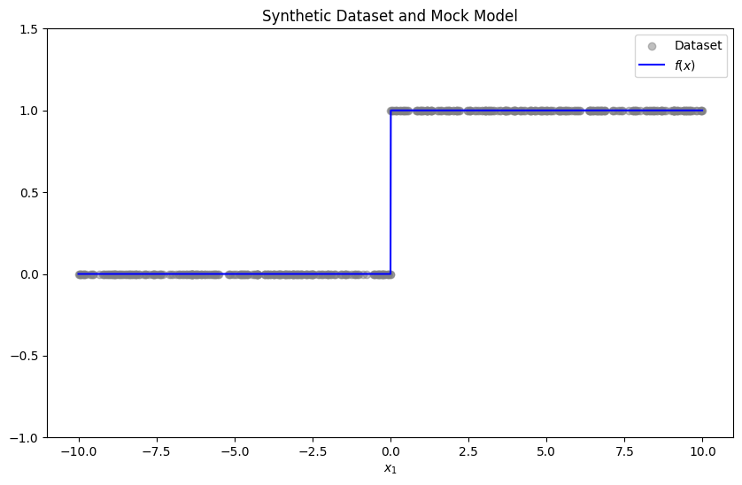

We have that

$$g(z)={\varphi }_0+\sum _{i=1}^M{\varphi }_i{z}_i={\varphi }_0+{\varphi }_{1}z$$

and thus

$$\begin{array}{rl}{\varphi }_0& =g(0)=f(\varnothing )\\ & \approx {\mathbb{E}}_x[f(x)].\end{array}$$

Furthermore, since we want

$$g(z^{\ast })=\sum _i{\varphi }_i={\varphi }_0+{\varphi }_1=f(x^{\ast }),$$

we have

$${\varphi }_1=f(x^{\ast })-{\varphi }_0\approx f(x^{\ast })-{\mathbb{E}}_x[f(x)].$$

Since 1-dimensional case is so simple, we can apply this for all $x^{\ast }\in \mathcal{D}$ and obtain a globally approximated surrogate $g$.

expected_value = np.mean(model_predictions)
shap_weights = model_predictions - expected_value
 
plt.figure(figsize=(10, 6))
plt.scatter(x_dataset, y_dataset, alpha=0.5, label='Dataset', color='gray')
 
plt.plot(x, model_predictions, label="$f(x)$", color='blue')
plt.axhline(y=expected_value, color='green', linestyle='--', label="$\phi_0 = \mathbb{E}_{x}[f(x)]$")
plt.plot(x, shap_weights, color='red', linestyle='--', label="$\phi_1=f(x^*)-\mathbb{E}_{x}[f(x)]$")
 
plt.ylim(-1, 1.5)
plt.title("SHAP Values for 1D Case")
plt.xlabel("$x_1$")
plt.legend()
plt.show()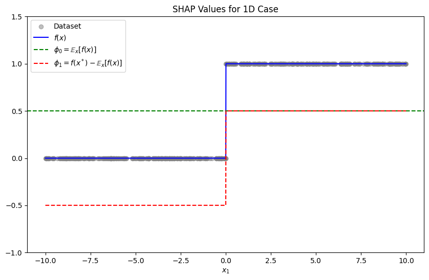

2-dimensional Case

Let us start by creating a synthetic dataset, and training a simple binary classifier to the dataset. We will use SVM as a classifier.

np.random.seed(RAND_SEED)
 
X, y = make_moons(n_samples=5000, noise=0.2, random_state=RAND_SEED)
X_train, X_test, y_train, y_test = train_test_split(
    X, y, test_size=0.3, random_state=RAND_SEED
)
 
instance_to_explain = X_test[10]
 
plt.figure(figsize=(10, 6))
plt.scatter(X_train[:, 0], X_train[:, 1], c=y_train, s=25, edgecolor='k', cmap=plt.cm.coolwarm)
plt.scatter(instance_to_explain[0], instance_to_explain[1], c='yellow', s=100, edgecolor='k', label='Instance to Explain')
plt.title("Synthetic Dataset")
plt.xlabel("$x_1$")
plt.ylabel("$x_2$")
plt.legend()
plt.show()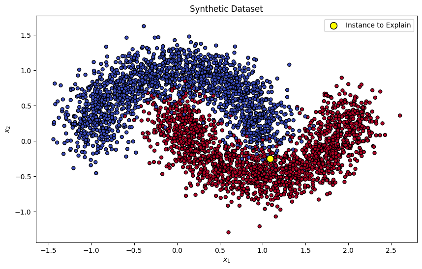

target_model = SVC(kernel='rbf', probability=True, random_state=RAND_SEED)
target_model.fit(X_train, y_train)
 
x_min, x_max = X[:, 0].min() - 1, X[:, 0].max() + 1
y_min, y_max = X[:, 1].min() - 1, X[:, 1].max() + 1
xx, yy = np.meshgrid(np.linspace(x_min, x_max, 100), np.linspace(y_min, y_max, 100))
 
Z = target_model.predict_proba(np.c_[xx.ravel(), yy.ravel()])[:, 1]
Z = Z.reshape(xx.shape)
 
plt.figure(figsize=(10, 6))
contour = plt.contourf(xx, yy, Z, levels=[0, 0.5, 1], cmap=plt.cm.coolwarm, alpha=0.4)
plt.scatter(X_train[:, 0], X_train[:, 1], c=y_train, s=15, edgecolor='k', cmap=plt.cm.coolwarm)
plt.scatter(instance_to_explain[0], instance_to_explain[1], c='yellow', s=100, edgecolor='k', label='Instance to Explain')
plt.title("Mock Model Decision Boundary")
plt.xlabel("$x_1$")
plt.ylabel("$x_2$")
plt.legend()
plt.show()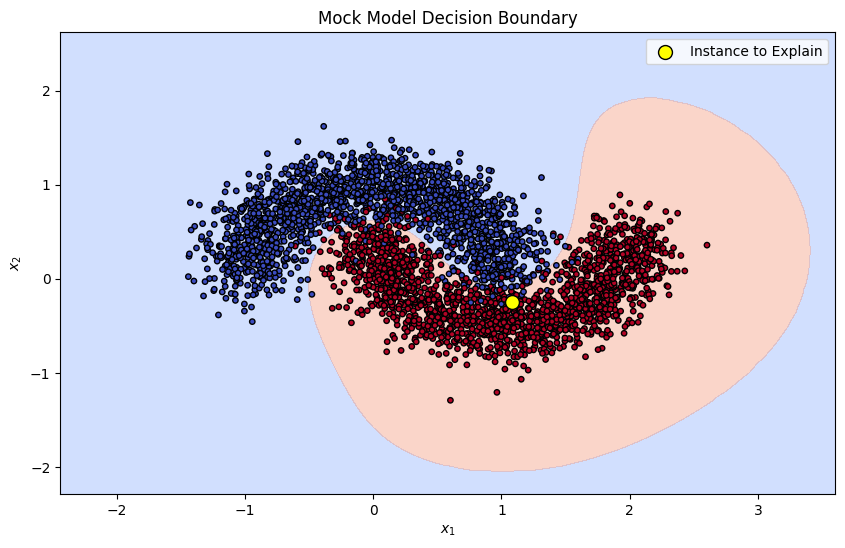

Given the shape of the dataset, we can anticipate that feature 2 would be the important factor when predicting the output of our instance of interest. Let’s see if SHAP values match our intuition!

We have that

$$g(z)=g((z_1,z_2))={\varphi }_0+\sum _{i=1}^M{\varphi }_i{z}_i={\varphi }_0+{\varphi }_1{z}_1+{\varphi }_2{z}_2$$

and thus

$$\begin{array}{rl}{\varphi }_0& =g((0,0))=f(\varnothing )\\ & \approx {\mathbb{E}}_{x_1,x_2}[f((x_1,x_2))].\end{array}$$

Now, we can apply the closed form formula for calculating the SHAP values:

$$\begin{array}{rl}{\varphi }_i& =\sum _{S\in F_i}\frac{|S|!(M-|S|-1)!}{M!}(f(h_{x^{\ast }}(z_{S\cup \{i\}}))-f(h_{x^{\ast }}(z_S)))\\ & \approx \sum _{S\in F_i}\frac{|S|!(M-|S|-1)!}{M!}({\mathbb{E}}_{x_{\overline{S\cup \{i\}}}}[f(x;x_{S\cup \{i\}}=x_{S\cup \{i\}}^{\ast })]-{\mathbb{E}}_{x_{\overline{S}}}[f(x;x_S=x_S^{\ast })])\end{array}$$

We can see that $F_1=\{\varnothing ,\{2\}\}$ and $F_2=\{\varnothing ,\{1\}\}$. Substituting the values yield:

$$\begin{array}{rl}{\varphi }_1& \approx \frac{1}{2}\left({\mathbb{E}}_{x_2}[f((x_1^{\ast },x_2))]-{\mathbb{E}}_{x_1,x_2}[f((x_1,x_2))]\right)\\ & +\frac{1}{2}\left(f((x_1^{\ast },x_2^{\ast }))-{\mathbb{E}}_{x_1}[f((x_1,x_2^{\ast }))]\right)\end{array}$$

and

$$\begin{array}{rl}{\varphi }_2& \approx \frac{1}{2}\left({\mathbb{E}}_{x_1}[f((x_1,x_2^{\ast }))]-{\mathbb{E}}_{x_1,x_2}[f((x_1,x_2))]\right)\\ & +\frac{1}{2}\left(f((x_1^{\ast },x_2^{\ast }))-{\mathbb{E}}_{x_2}[f((x_1^{\ast },x_2))]\right)\end{array}$$

We only need to compute three expected values: ${\mathbb{E}}_{x_1,x_2}[f((x_1,x_2))]$, ${\mathbb{E}}_{x_1}[f((x_1,x_2^{\ast }))]$, and ${\mathbb{E}}_{x_2}[f((x_1^{\ast },x_2))]$.

Let us start by computing ${\mathbb{E}}_{x_1,x_2}[f((x_1,x_2))]$.

train_probabilities = target_model.predict_proba(X_train)[:, 1]
phi_0 = np.mean(train_probabilities)
 
math_print(fr"$\phi_0 \approx \mathbb{{E}}_{{x_1, x_2}} [f((x_1, x_2))] = {phi_0}$")

$$\text{Result: }{\varphi }_0\approx {\mathbb{E}}_{x_1,x_2}[f((x_1,x_2))]=0.49622315331032374$$

Next, we will calculate the marginal expectations.

plt.figure(figsize=(10, 6))
plt.scatter(X_train[:, 0], X_train[:, 1], c=y_train, s=25, edgecolor='k', alpha=0.4, cmap=plt.cm.coolwarm)
plt.scatter(instance_to_explain[0], instance_to_explain[1], c='yellow', s=100, edgecolor='k', label='Instance to Explain')
 
plt.axvline(x=instance_to_explain[0], color='grey', linewidth=5, alpha=0.7)
plt.axhline(y=instance_to_explain[1], color='grey', linewidth=5, alpha=0.7)
 
plt.title("Marginalisation Demonstration")
plt.xlabel("$x_1$")
plt.ylabel("$x_2$")
plt.legend()
plt.show()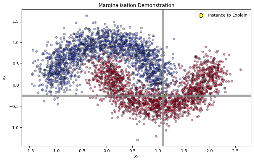

x1_replaced = np.array([[x[0], instance_to_explain[1]] for x in X_train])
x2_replaced = np.array([[instance_to_explain[0], x[1]] for x in X_train])
 
x1_replaced_probabilities = np.mean(target_model.predict_proba(x1_replaced)[:, 1])
x2_replaced_probabilities = np.mean(target_model.predict_proba(x2_replaced)[:, 1])
 
math_print(fr"$\mathbb{{E}}_{{x_1}} [f((x_1, x^*_2))] = {x1_replaced_probabilities}\\ \mathbb{{E}}_{{x_2}} [f((x^*_1, x_2))] = {x2_replaced_probabilities}$")

$$\begin{array}{rl}& \text{Results: }\\ & {\mathbb{E}}_{x_1}[f((x_1,x_2^{\ast }))]=0.8171045461221259\\ & {\mathbb{E}}_{x_2}[f((x_1^{\ast },x_2))]=0.2996089774564694\end{array}$$

Finally, we can compute the SHAP values.

instance_to_explain_probability = target_model.predict_proba([instance_to_explain])[0, 1]
 
phi_1 = 0.5 * (instance_to_explain_probability - x1_replaced_probabilities + x2_replaced_probabilities - phi_0)
phi_2 = 0.5 * (instance_to_explain_probability - x2_replaced_probabilities + x1_replaced_probabilities - phi_0)
 
math_print(fr"$\phi_0 = {phi_0}\\ \phi_1 = {phi_1}\\ \phi_2 = {phi_2}$")

$$\begin{array}{rl}& \text{Results: }\\ & {\varphi }_0=0.49622315331032374\\ & {\varphi }_1=-0.05289198605052847\\ & {\varphi }_2=0.46460358261512796\end{array}$$

Each ${\varphi }_i$ is the contribution of feature $i$ towards the model output. We can interpret the SHAP values as follows:

• The first feature $x_1$ has a negative contribution of $-0.05$: this feature is negatively correlated with the prediction of the model for this instance. For similar examples with different values of $x_1$, the prediction of the model would be sightly larger.
• The second feature $x_2$ has a negative contribution of $0.46$: this feature is positively correlated with the prediction of the model for this instance.

We can see numerically that feature 2 has a much larger positive contribution when predicting through our mock model. This matches our intuition given the shape of the dataset!

(28 $\times$ 28)-dimensional Case: MNIST Dataset

However, there still remains a problem when approximating Shapley values: what if the dimension $M$ is too large? To overcome this problem, the authors of SHAP proposed an improvement to LIME in order to maintain the desired property of Shapley values.

According to the authors, “the answer depends on the choice of loss function $\mathcal{L}$, weighting kernel (proximity function) ${\pi }_x$ and regularisation term $\Omega$.” In LIME, choices for these parameters are made heuristically, leading to sub-par result that does not satisfy all the desired properties:

$$\begin{array}{rl}\Omega (g)& =(\text{Complexity of }g)\\ {\pi }_x^{\text{LIME}}(z)& =\exp (-D(x,z{)}^2/{\sigma }^2)\\ \mathcal{L}(f,g,{\pi }_x^{\text{LIME}})& =\sum _{z,z^{\prime }\in \mathcal{Z}}{\pi }_x^{\text{LIME}}(z){\left(f(z)-g(z^{\prime })\right)}^2\end{array}$$

Instead, the authors have found the appropriate loss function $\mathcal{L}$, weighting kernel ${\pi }_x$ and regularisation term $\Omega$ that is capable of properly recovering the Shapley values:

$$\begin{array}{rl}\Omega (g)& =0\\ {\pi }_x^{\text{SHAP}}(z_S)& =\frac{M-1}{\left(\genfrac{}{}{0ex}{}{M}{|S|}\right)\cdot |S|\cdot (M-|S|)}\\ \mathcal{L}(f,g,{\pi }_x^{\text{SHAP}})& =\sum _{S\in F}{\pi }_x^{\text{SHAP}}(z_S){\left(f(h_x(z_S))-g(z_S)\right)}^2\\ & \approx \sum _{S\in F}{\pi }_x^{\text{SHAP}}(z_S){\left({\mathbb{E}}_{x_{\overline{S}}}[f(x;x_S=x_S^{\ast })]-g(z_S)\right)}^2\end{array}$$

Linear regression with this weighting kernel yields a good approximation on the Shapley values, turning the complex problem of calculating the Shapley values into a simple linear regression problem!

If the dataset $\mathcal{D}$ is too large, we can also limit the number of samples when calculating the expected values. We can select coalitions a little more strategically. We can see that the KernelSHAP weighting function, ${\pi }_x^{\text{SHAP}}$, emphasises coalitions that either include just a few features or nearly all of them. This approach is used because focusing on a small number of features helps to show how each feature operates independently. On the other hand, considering almost all features at once helps to demonstrate how they work together and influence each other. By prioritising the sampling from these specific groups instead of randomly choosing feature groups, we can get a more accurate approximation of Shapley values.

def shap_weighting_kernel(z, p):
    return (p-1)/(binom(p, z)*(z*(p-z)))
 
n_features = 28*28
 
x = list(range(1, n_features))
kernel_shap_weights = [shap_weighting_kernel(z, n_features) for z in x]
 
plt.figure(figsize=(10, 6))
plt.plot(x, kernel_shap_weights, label="KernelSHAP Weight")
plt.yscale('log')
plt.title(f"KernelSHAP Weights for ${n_features}$ Features")
plt.xlabel("Number of features $|S|$")
plt.ylabel("Weight (log scaled)")
plt.legend()
plt.show();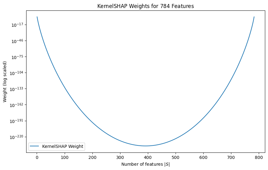

Given these, let us train a simple neural network on the MNIST dataset and explain its output using KernelSHAP.

device = torch.device("cuda" if torch.cuda.is_available() else "cpu")
transform = transforms.Compose([transforms.ToTensor(),
                                transforms.Normalize((0.5,), (0.5,))])
 
trainset = torchvision.datasets.MNIST(root='./data', train=True, download=True, transform=transform)
trainloader = torch.utils.data.DataLoader(trainset, batch_size=64, shuffle=True)
 
testset = torchvision.datasets.MNIST(root='./data', train=False, download=True, transform=transform)
testloader = torch.utils.data.DataLoader(testset, batch_size=64, shuffle=False)

class Net(nn.Module):
    def __init__(self):
        super(Net, self).__init__()
        self.fc1 = nn.Linear(28 * 28, 128)
        self.fc2 = nn.Linear(128, 64)
        self.fc3 = nn.Linear(64, 10)
 
    def forward(self, x):
        x = x.view(-1, 28 * 28)
        x = torch.relu(self.fc1(x))
        x = torch.relu(self.fc2(x))
        x = self.fc3(x)
        return x
 
model = Net().to(device)
criterion = nn.CrossEntropyLoss()
optimizer = torch.optim.Adam(
    model.parameters(), lr=1e-3, betas=(0.9, 0.999), weight_decay=0.01
)
 
model.train()
for epoch in range(5):
    for i, data in enumerate(trainloader, 0):
        inputs, labels = data[0].to(device), data[1].to(device)
 
        optimizer.zero_grad()
 
        outputs = model(inputs)
        loss = criterion(outputs, labels)
        loss.backward()
        optimizer.step()
 
        if i % 200 == 0:
            print(f"[{epoch + 1}, {i:4d}] loss: {loss.item():.3f}")

def predict(data):
    data_tensor = torch.tensor(data, dtype=torch.float32).to(device)
    model.eval()
 
    with torch.no_grad():
        output = model(data_tensor)
 
    return output.cpu().numpy()
 
batch = next(iter(testloader))
images, _ = batch
 
num_images = 5
test_images = images[:num_images].view(num_images, -1).cpu().numpy()
 
explainer = shap.KernelExplainer(predict, shap.kmeans(test_images, 5))
shap_values = explainer.shap_values(test_images, nsamples=10000)
shap_values = [x.reshape(num_images, 28, 28) for x in shap_values]
 
num_images = len(test_images)
num_classes = len(shap_values)
 
max_shap = max(abs(shap_value).max() for shap_value_group in shap_values for shap_value in shap_value_group)
fig, axes = plt.subplots(num_images, num_classes + 1, figsize=(12, 1.5 * num_images))
 
for i in range(num_images):
    axes[i, 0].imshow(test_images[i].reshape(28, 28), cmap='gray')
    axes[i, 0].axis('off')
    if i == 0:
        axes[i, 0].set_title('Original Image')
 
    for j in range(num_classes):
        shap_image = shap_values[j][i]
        mappable = axes[i, j + 1].imshow(shap_image, cmap='seismic', vmin=-max_shap, vmax=max_shap)
        axes[i, j + 1].axis('off')
        if i == 0:
            axes[i, j + 1].set_title(f'Class {j}')
 
plt.tight_layout(pad=0.4, w_pad=0.5, h_pad=0.2)
plt.subplots_adjust(bottom=0.1)
cbar_ax = fig.add_axes([0.15, 0.05, 0.7, 0.02])
fig.colorbar(mappable, cax=cbar_ax, orientation='horizontal')
plt.show()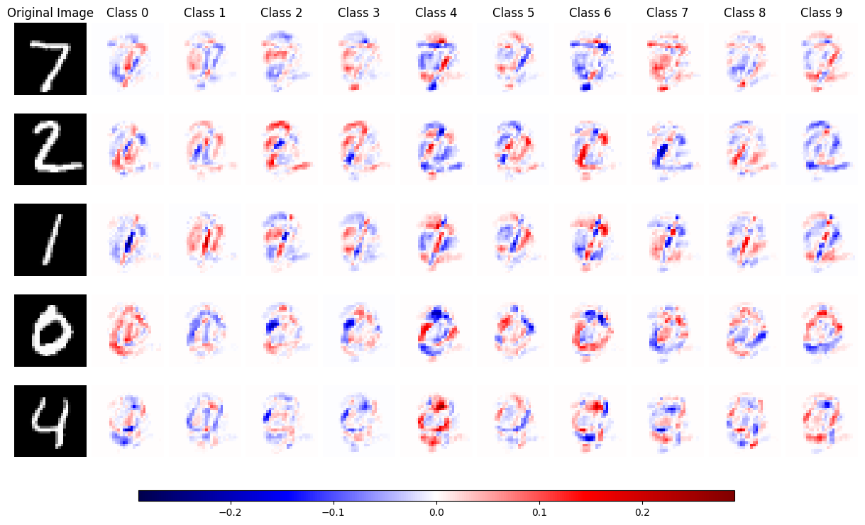

The red colour indicates a positive SHAP value, where blue indicates a negative SHAP value.

Conclusion

In this project, we explored the critical domain of explainable AI (XAI), focusing on interpreting machine learning models through advanced techniques that utilises surrogate models, specifically LIME and SHAP.

We explored how LIME uses local surrogate models—ridge regression, in particular—to explain complex model predictions in a localised context. This strategy successfully achieved a balance between maintaining the original model’s decisions and the requirement for interpretability.

We then turned to SHAP and studied its game-theoretic foundations to distribute feature importance fairly. We also showed how these XAI techniques may clarify the decision-making processes of complex algorithms, making AI more transparent and approachable through real-world applications on datasets like as MNIST.

Our exploration of XAI highlights its key role in making AI ethical and understandable. Techniques like LIME and SHAP help us better understand complex AI models, ensuring they align with our values and ethics. As AI becomes more common in our lives, these methods become even more important, helping AI to be a positive and beneficial tool for society.

References

• Das, A., & Rad, P. (2020). Opportunities and challenges in explainable artificial intelligence (XAI): A survey. arXiv preprint arXiv:2006.11371.
• Goodfellow, I. J., Shlens, J., & Szegedy, C. (2014). Explaining and harnessing adversarial examples. arXiv preprint arXiv:1412.6572.
• Lapuschkin, S. (2019). Opening the machine learning black box with layer-wise relevance propagation.
• Heaven, W. D. (2021, July 30). Hundreds of AI Tools Have Been Built to Catch Covid. None of Them Helped. MIT Technology Review. https://www.technologyreview.com/2021/07/30/1030329/machine-learning-ai-failed-covid-hospital-diagnosis-pandemic/.
• Bach, S., Binder, A., Montavon, G., Klauschen, F., Müller, K. R., & Samek, W. (2015). On pixel-wise explanations for non-linear classifier decisions by layer-wise relevance propagation. PloS one, 10(7), e0130140.
• Montavon, G., Binder, A., Lapuschkin, S., Samek, W., & Müller, K. R. (2019). Layer-wise relevance propagation: an overview. Explainable AI: interpreting, explaining and visualizing deep learning, 193-209.
• Kim, S. W., Kang, S. H., Kim, S. J., & Lee, S. (2021). Estimating the phase volume fraction of multi-phase steel via unsupervised deep learning. Scientific Reports, 11(1), 5902.
• Montavon, G., Lapuschkin, S., Binder, A., Samek, W., & Müller, K. R. (2017). Explaining nonlinear classification decisions with deep taylor decomposition. Pattern recognition, 65, 211-222.
• Ribeiro, M. T., Singh, S., & Guestrin, C. (2016, August). ” Why should i trust you?” Explaining the predictions of any classifier. In Proceedings of the 22nd ACM SIGKDD international conference on knowledge discovery and data mining (pp. 1135-1144).
• Molnar, C. (2022). Interpretable machine learning: A guide for making Black Box models explainable. Christoph Molnar.
• López, S., & Saboya, M. (2009). On the relationship between Shapley and Owen values. Central European Journal of Operations Research, 17, 415-423.
• Owen, G. (1977). Values of games with a priori unions. In Mathematical economics and game theory: Essays in honor of Oskar Morgenstern (pp. 76-88). Springer Berlin Heidelberg.
• Wagner, L. (2022, May 21). Shap’s partition explainer for language models. Medium. https://towardsdatascience.com/shaps-partition-explainer-for-language-models-ec2e7a6c1b77
• Thiebaut, N. (2020, February 29). Understanding the shap interpretation method: Kernel shap. Data4thought. https://data4thought.com/kernel_shap.html
• Winastwan, R. (2021, January 20). Interpreting image classification model with lime. Medium. https://towardsdatascience.com/interpreting-image-classification-model-with-lime-1e7064a2f2e5
• Shapley, L. S. (1953). A value for n-person games.
• Štrumbelj, E., & Kononenko, I. (2014). Explaining prediction models and individual predictions with feature contributions. Knowledge and information systems, 41, 647-665.
• Sundararajan, M., & Najmi, A. (2020, November). The many Shapley values for model explanation. In International conference on machine learning (pp. 9269-9278). PMLR.
• Janzing, D., Minorics, L., & Blöbaum, P. (2020, June). Feature relevance quantification in explainable AI: A causal problem. In International Conference on artificial intelligence and statistics (pp. 2907-2916). PMLR.
• Marcotcr. MARCOTCR/Lime: Lime: Explaining the predictions of any machine learning classifier. GitHub. https://github.com/marcotcr/lime
• Slundberg. Slundberg/SHAP: A game theoretic approach to explain the output of any machine learning model. GitHub. https://github.com/slundberg/shap